Course notes on differential privacy

Mon 28 June 2021

This article contains my course notes for Secure and Private AI offered by Udacity.

Definitions

Differential Privacy is a measure of how much information is leaked when querying a database. An intuition for privacy is constructed from the following building blocks:

1) An initial database (e.g a binary Pytorch tensor).

import torch
def init_db(num_entries = 5000):
   return torch.rand(num_entries) > 0.5

2) A set of n parallel databases. These are copies of the initial database with an element removed.

from copy import copy

def get_parallel_db(db, remove_index):
   return torch.cat((db[:remove_index], db[remove_index+1:]))

def parallel_dbs(db):
   dbs = []

   for i in range(len(db)):
       dbs.append(get_parallel_db(db, i))
   return dbs

Queries on this database, and its parallels, are operations on its elements. In the lectures we worked with tensors, arithmetics (sum()) and simple statistics (mean()). In practice, these could be aggregation queries in a relational database, or stochastic functions in the training of a machine learning model.

Evaluating the privacy of a function

To evaluate if a query is leaking private information, we calculate the maximum amount of change when it is performed on all parallel databases. This metric is called sensitivity. In the lectures, and literature, sensitivity is expressed in terms the L1 norm. A bit more formally, if \(X\) is the original database and \(x_a, x_b\) its parallels, the sensitivity of a query \(q\) is defined as

Experimentally, we learn that the mean() query has lower sensitivity than the sum() query. As a third example we examine the senstivity of a threshold() function.

Finally, we show that none of these functions are differentially private by performing an adversarial attack on them.

# create a database
db, _ = create_db_and_parallels(5000)

# we look at the value of row 10 (arbitrarly picked)
db[10]
# We discard row 10, and perform a number of attacks on the parallel dbs to recover its value.
pdb = get_parallel_db(db, remove_index=10)

# Attack against the sum() query
th = db.sum() - 1
# This should match the (private) value of db[10].
# We recovered the original item from the aggerate results.
(db.float().sum() > th).float() - (pdb.float().sum() > th).float()

The set of queries we just performed to reconstruct the original database is referred to as a differencing attack. It follows that a degree of randomness is necessary to satisfy privacy constraints.

Local vs Global privacy

Depending on when randomness is added, we distinguish between local and global differential privacy. With local privacy we add noise to each individial data point. With global privacy, we add noise to the query.

Both methods have tradeoffs. Notably global DP is computationally tractable, and possibly more accurate, but requires us to trust the database owner and that no datapoint was observed before the query took place. Computationally more expensive local DP might be necessary when data is so sensitive, that we do not trust that noise will be added after observing it.

Randomized Response is given as an example of local privacy.

Epsilon-delta differential privacy

Global differential privacy is expressed in tems of the epsilon-delta theorem ¹:

Given a randomized algorithm \(M\) with domain \(\mathbb{N}^{|\chi|}\) (e.g. histograms over a database). \(\forall S \subseteq Range(M), \forall x, y \in \mathbb{N}^{|\chi|}\) s.t. \(|| x -y || \leq 1\) (\(x\), \(y\) are parallel databases).

If \(\delta = 0\), we say that \(M\) is \(\epsilon\)-differentially private.

This formalism expresses a query in terms of a "randomized algorithm" \(M\). The equation measures how much privacy is afforded by \(M\), by comparing running \(M\) on an initial database \(x\) and parallel database \(y\).

\(\epsilon\) controls the maximum distance between \(x\) and \(y\). \(\delta\) is the probability that the \(\epsilon\) constraint won't hold. Tradeoffs between \(\epsilon\) and \(\delta\) control privacy.

Adding noise to the "randomized algorithm"

The amount of noise to apply to the query \(M\) is a function of

1. The type of noise (e.g Gaussian, Laplacian).
2. The sensitivity of the query function.
3. The desired \(\epsilon\).
4. The desired \(\delta\).

The following example shows how noise can be added to a sum() query. The noise is sampled from a \(Laplace (\mu, \beta)\) distribution. The desired \(\epsilon\), and sensitivity of the query, determine the parametrisation of the Laplacian (e.g. \(\beta = \frac{sensitivity}{\epsilon}\)). In literature, this approach is referred to as Laplace Meachanism. It has some nice theoretical properties that, in the general case, ensure that \(\delta = 0\) ².

epsilon = 0.5
db, pdbs = create_db_and_parallels(5000)

# Randomised algorithm that adds Laplacian noise to a query
def M(db, query, sensitivy):
    b = sensitivy / epsilon 
    noise = torch.tensor(np.random.laplace(0, b, 1))
    return query(db) + noise
# Sensitivity for `sum` query is 1
def query(db):
    return db.sum()

sensitivity(query, 5000)
M(db, query, 1), query(db)

Training private ML models

In the reminder of the course we build on this definition of DP to train private machine learning models. The problem we want to solve is to minimize the amount of information leak in a public set of predictions, and thus protect our model from adversarial attacks (e.g. differencing attacks). See Rigaki & Garcia, A Survey of Privacy Attacks in Machine Learning, 2021 for an introduction on this topic.

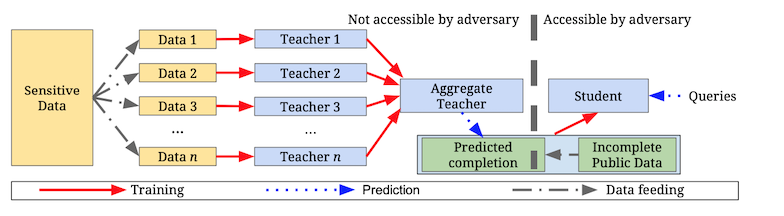
We use the Private Aggregation of Teacher Ensembles (PATE) framework to learn from private data. PATE assumes two main components: private labelled datasets ("teachers") and a public unlabelled dataset ("student").

Private data is partitioned in non-overlapping training sets. An ensamble of "teachers" are trained independently (with no privacy guarantee). The "teacher" models are scored on the unlabelled, public, "student" datasets. Their predictions are aggregated and perturbed with random noise. A "student" model can then trained on public data labelled by the ensamble, instead of on the original, private, dataset.

An example of this training scheme can be found at https://github.com/gmodena/tinydp.

A-posteriori analysis is performed on the teachers aggregate to determie whether the model satisfies the desired \(\epsilon\) budget. In the course we used the pysyft package for this.

from syft.frameworks.torch.dp import pate

data_dep_eps, data_ind_eps = pate.perform_analysis(teacher_preds=preds,
                                                   indices=student_labels,
                                                   noise_eps=epsilon, delta=1e-5)
print("Data Independent Epsilon:", data_ind_eps)
print("Data Dependent Epsilon:", data_dep_eps)

perform_analysis() uses teacher data, true labels, and a moment tracking algorithm, to compute two metrics:

• a data dependent epsilon quantifies models agreement.
• an epsilon value independet of data, that shows the maximum amount of privacy that could be leaked.

Intuitively, the more models agree (and overfit less), the less privacy they will leak (thus the lower data dependent epsilon). As a corollary, it is observed that good privacy is obtained by models that generalise and do not overfit.

Troubleshooting pysyft dependencies

Installing pysyft and the right dependencies for pate on macOS has been a bit tricky. After some tweaking, I was able to set things up with this conda environment.